
Text Classification
Over the years I have given many presentations about how to use machine learning to classify text documents. I wanted to create a notebook that would serve as a template for such presentations, allowing me to quickly demonstrate the process of text classification using machine learning techniques. The problem of text classification is a common task in natural language processing, where the goal is to assign predefined categories to text documents based on their content. This notebook demonstrates how to classify documents from the 20 Newsgroups dataset using a decision tree classifier. We will preprocess the text data, extract features using a bag-of-words model, train a classifier, and evaluate its performance.
import matplotlib.pyplot as plt
import pandas as pd

from sklearn.datasets import fetch_20newsgroups
from sklearn.feature_extraction.text import CountVectorizer
from sklearn.tree import DecisionTreeClassifier

from sklearn.tree import plot_tree
loading the dataset
For this demonstration we will use the 20 Newsgroups dataset. We will load the data and show an example of a document from each category.
categories = [
    'rec.motorcycles',
    'rec.sport.baseball',
    'comp.graphics',
    'sci.space',
]

remove = ('headers', 'footers', 'quotes')

data_train = fetch_20newsgroups(subset='train', categories=categories,
                                shuffle=True, random_state=42,
                                remove=remove)

data_test = fetch_20newsgroups(subset='test', categories=categories,
                               shuffle=True, random_state=42,
                               remove=remove)
print('data loaded')
# order of labels in `target_names` can be different from `categories`
target_names = data_train.target_names


def size_mb(docs):
    return sum(len(s.encode('utf-8')) for s in docs) / 1e6

data_train_size_mb = size_mb(data_train.data)
data_test_size_mb = size_mb(data_test.data)

print("%d documents - %0.3fMB (training set)" % (
    len(data_train.data), data_train_size_mb))
print("%d documents - %0.3fMB (test set)" % (
    len(data_test.data), data_test_size_mb))

df = pd.DataFrame()
df['text'] = data_train.data
df['target'] = [data_train.target_names[x] for x in data_train.target]
df.head()

for category in categories:
    df_category = df[df['target'] == category]
    print(f"=========================={category}==========================")
    print(df_category['text'].values[0][:500])
    data loaded
    2372 documents - 2.170MB (training set)
    1578 documents - 1.576MB (test set)
    ==========================rec.motorcycles==========================

      Why not?  Ford owns Aston-Martin and Jaguar, General Motors owns Lotus
    and Vauxhall.  Rover is only owned 20% by Honda.

    -----------------------------------------------------------------------------
    ==========================rec.sport.baseball==========================
    Subject line says it all. Thanks in advance. Please email
    chuck@cygnus.eid.anl.gov
    Go Cubs!

    ==========================comp.graphics==========================
    A shareware graphics program called Pman has a filter that makes a picture
    look like a hand drawing.  This picture could probably be converted into
    vector format much easier because it is all lines. (With Corel Trace, etc..)

    ==========================sci.space==========================
    Could someone please send me the basics of the NASP project:
    1. The proposal/objectives
    2. The current status of the project/obstacles encountered
    3. Chance that the project shall ever be completed
    or any other interesting information about this project.

    Any help will be much appreciated
bag of words vectorization
We will use a CountVectorizer to convert the text documents into a matrix of word counts. Each row in the matrix corresponds to a document, and each column corresponds to a word in the vocabulary. The value in each cell represents the count of that word in the corresponding document. In this case we only use words that appear at least 2 times and ignore stop words like “the”, “is”, etc.
To illustrate, first use a simple example:
sentences = [
    "The cat sat on the mat.",
    "The dog chased the cat.",
    "The mat was sat on by the dog."
]
vectorizer = CountVectorizer(stop_words='english', min_df=2)
X_train = vectorizer.fit_transform(sentences)
X_train_df = pd.DataFrame(X_train.toarray(), columns=vectorizer.get_feature_names_out())
X_train_df.insert(0, 'sentence', sentences)
print("n_samples: %d, n_features: %d" % X_train.shape)
print(X_train_df)
    n_samples: 3, n_features: 4
                             sentence  cat  dog  mat  sat
    0         The cat sat on the mat.    1    0    1    1
    1         The dog chased the cat.    1    1    0    0
    2  The mat was sat on by the dog.    0    1    1    1
now do the same for the training data
vectorizer = CountVectorizer(stop_words='english', min_df=3) #only use words that appear at least 3 times
X_train = vectorizer.fit_transform(data_train.data)
print("n_samples: %d, n_features: %d" % X_train.shape)
n_samples: 2372, n_features: 8312
training a decision tree classifier
We will train a DecisionTreeClassifier on the training data. The DecisionTreeClassifier is a simple yet effective algorithm for classification tasks. It works by recursively splitting the data based on the features, creating a tree-like structure where each node represents a feature and each leaf node represents a class label. The advantage of decision trees is that they are easy to interpret and visualize, making them a good choice for understanding the classification process.
classifier = DecisionTreeClassifier(max_depth=4,
                                    random_state=42,
                                    min_samples_leaf=10)

classifier.fit(X_train, data_train.target)

# plot the tree
plt.figure(figsize=(20, 10))
plot_tree(classifier, filled=True, feature_names=vectorizer.get_feature_names_out(),
           class_names=target_names)
plt.show()
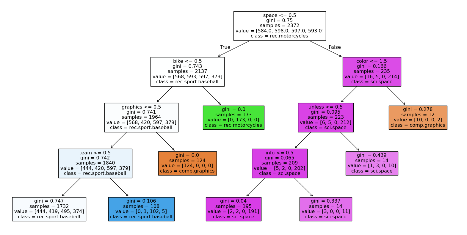
If we plot the tree we can see how the decision tree splits the data based on the features. Each node in the tree represents a feature, and the branches represent the decisions made based on the values of those features. The gini impurity is a measure of how often a randomly chosen element from the set would be incorrectly labeled if it was randomly labeled according to the distribution of labels in the subset. A lower gini impurity indicates a better split, as it means that the classes are more homogeneous. Samples means the number of samples in the node, and value shows the distribution of classes in that node. Class shows the predicted class for that node.
For example the first node splits the data on the word “space”. If it occurs less than 0.5 times in the document, it goes to the left child node, otherwise it goes to the right child node.
making predictions
Now that we have the model, we can use it to make predictions on the test data. First we will transform the test data using the same CountVectorizer that we used for the training data. This ensures that the features are consistent between the training and test sets. Then we will use the trained classifier to predict the classes of the test documents.
X_test = vectorizer.transform(data_test.data)
print("n_samples: %d, n_features: %d" % X_test.shape)
y_pred = classifier.predict(X_test)
print(y_pred)
n_samples: 1578, n_features: 8312
[2 2 1 ... 2 1 2]
evaluating the classifier
Finally we will evaluate the performance of the classifier. The confusion matrix shows a table where each row represents the true class and each column represents the predicted class. The diagonal elements represent the number of correct predictions, while the off-diagonal elements represent the misclassifications. The classification report provides additional metrics such as precision, recall, and F1-score for each class, giving a more detailed view of the classifier’s performance.
#plot the confusion matrix
from sklearn.metrics import ConfusionMatrixDisplay
from sklearn.metrics import classification_report

ConfusionMatrixDisplay.from_estimator(classifier, X_test, data_test.target,
                                       display_labels=[t.split(".")[-1] for t in target_names],
                                       cmap=plt.cm.Blues,
                                       normalize='true')
plt.show()
# make classification report
print(classification_report(data_test.target, y_pred, target_names=target_names))

                        precision    recall  f1-score   support

         comp.graphics       0.98      0.26      0.41       389
       rec.motorcycles       1.00      0.26      0.41       398
    rec.sport.baseball       0.32      0.99      0.48       397
             sci.space       0.84      0.30      0.44       394

              accuracy                           0.45      1578
             macro avg       0.78      0.45      0.43      1578
          weighted avg       0.78      0.45      0.43      1578
The performance of this model is not very good, with an accuracy of around 0.5. This is expected given the simplicity of the decision tree classifier and the complexity of the text data. However, it serves as a good starting point for understanding how to approach text classification tasks using machine learning techniques. For more advanced models, we could consider using other features such as TF-IDF, or more complex classifiers like Random Forests or xgboost. Also NLP techniques like word embeddings with word2vec, or language parsers like spacy could be used to improve the performance of the model.